Using skrmdb

Notation

The methods of Spearman-Karber, Reed-Muench, and Dragstedt-Behrens are all commonly used to estimate ED50. In what follows, we use the following variable notation:

x is a vector corresponding to the log dilution or dose for each group.
n is an integer vector corresponding to the group size at each log dilution or dose.
y is an integer vector corresponding to the number responding at each log dilution or dose.

All examples are with SpearKarb(), however, the usage for DragBehr() and ReedMuench() is identical.

Usage

Each of the main functions in skrmdb can be called in three different ways.

To illustrate this, we start with a simple data set where the number of dead increases with the dosage.

dead <- c(0, 3, 5, 8, 10, 10)
total <- rep(10, 6)
dil <- 1:6

First we use the historical, deprecated, function call.

SpearKarb(y = dead, n = total, x = dil)

## Warning: skrmdb :: Calling this function with the parameters y, n, x is
## depreciated.

## ED50 by the Spearman-Karber method
## ed:   2.9

## Count trend is increasing with dilution.

The preferred method is to use formulas in the function call.

We can use the formula on the individual vectors.

SpearKarb(dead + total ~ dil)

## ED50 by the Spearman-Karber method
## ed:   2.9

## Count trend is increasing with dilution.

We can also use the formula on columns in a data.frame.

data <- data.frame(y = dead, n = total, x = dil)
SpearKarb(y + n ~ x, data)

## ED50 by the Spearman-Karber method
## ed:   2.9

## Count trend is increasing with dilution.

Method Assumptions

Each of these methods was designed to work under the assumption that x is either increasing or decreasing and y / n is increasing with the index.

It was decided that the functions DragBehr(), ReedMuench(), and SpearKarb() will sort the data for you according to this assumption.

To illustrate this, we create some data that is descending according to dilution.

dead <- c(10, 10, 8, 5, 3, 0)
total <- rep(10, 6)
dil <- 1:6

And we see that no mater how we enter the data, the same ED50 is reported.

SpearKarb(dead + total ~ dil)

## ED50 by the Spearman-Karber method
## ed:   4.1

## Count trend is decreasing with dilution.

SpearKarb(rev(dead) + rev(total) ~ rev(dil))

## ED50 by the Spearman-Karber method
## ed:   4.1

## Count trend is decreasing with dilution.

However, if we can decided to turn off the autosort, which will give us a different, but incorrect, estimate of ED50.

SpearKarb(dead + total ~ dil, autosort = FALSE)

## ED50 by the Spearman-Karber method
## ed:   2.9

## Count trend is decreasing with dilution.

Conditional ED50

The function skrmdb.all returns the ED50 for the three methods, along with additional data about the data sets that may be of interest.

For this section, we use the example data set titration. This data.frame contains the results of a hypothetical experiment where the ED50 of three vials (numbered 1, 2, 3) were each tested by three anonymous operators (TK, NU, CT).

head(titration)

##   testID   PrepID PrepRole      Date Vial Operator   dil positive total
## 1   BRSV BRSV-001     test 03-Mar-19    1       TK 1e-02       10    10
## 2   BRSV BRSV-001     test 03-Mar-19    1       TK 1e-03       10    10
## 3   BRSV BRSV-001     test 03-Mar-19    1       TK 1e-04        9    10
## 4   BRSV BRSV-001     test 03-Mar-19    1       TK 1e-05        6    10
## 5   BRSV BRSV-001     test 03-Mar-19    1       TK 1e-06        1    10
## 6   BRSV BRSV-001     test 03-Mar-19    1       TK 1e-07        1    10

First we need to compute the log dilution.

titration$log_dil <- -log10(titration$dil)

Plotting the data shows us that the tests visually seem to give roughly the same ED50, but unfortunately, there are missing data points.

ggplot(titration, aes(x = log_dil, y = positive)) +
  geom_point() +
  facet_grid(Vial ~ Operator) +
  geom_line()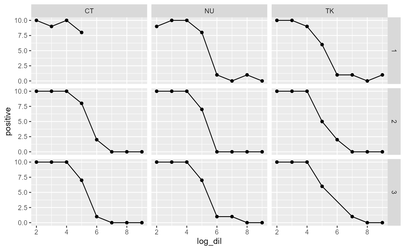

Nine plots showing titration data.

We could find ED50 by aggregation the data from all 9 tests for each of the three methods.

skrmdb.all(positive + total ~ log_dil, titration)

##   DragBehr ReedMuench SpearKarb SpearKarb.var response.increasing
## 1 5.365201   5.331023  5.332341   0.005014876               FALSE
##   duplicate.dilutions even.dilution monotonic bracket.midpoint
## 1                TRUE          TRUE      TRUE             TRUE

We can also see if there is a difference between Operators;

skrmdb.all(positive + total ~ log_dil | Operator, titration)

##   Operator DragBehr ReedMuench SpearKarb SpearKarb.var response.increasing
## 1       TK 5.286004   5.247059  5.283333    0.01954578               FALSE
## 2       NU 5.376350   5.340000  5.333333    0.01222222               FALSE
## 3       CT 5.418526   5.402062  5.383333    0.01399022               FALSE
##   duplicate.dilutions even.dilution monotonic bracket.midpoint
## 1                TRUE          TRUE     FALSE             TRUE
## 2                TRUE          TRUE     FALSE             TRUE
## 3                TRUE          TRUE     FALSE             TRUE

Or by Vial;

skrmdb.all(positive + total ~ log_dil | Vial, titration)

##   Vial DragBehr ReedMuench SpearKarb SpearKarb.var response.increasing
## 1    1 5.405272   5.377551  5.383333    0.02231347               FALSE
## 2    2 5.339806   5.304348  5.300000    0.01164751               FALSE
## 3    3 5.360000   5.319149  5.333333    0.01454527               FALSE
##   duplicate.dilutions even.dilution monotonic bracket.midpoint
## 1                TRUE          TRUE      TRUE             TRUE
## 2                TRUE          TRUE      TRUE             TRUE
## 3                TRUE          TRUE      TRUE             TRUE

Or by Operator and Vial.

skrmdb.all(positive + total ~ log_dil | Vial + Operator, titration)

##   Vial Operator DragBehr ReedMuench SpearKarb SpearKarb.var response.increasing
## 1    1       TK 5.306306   5.266667      5.30    0.06666667               FALSE
## 2    1       NU 5.429825   5.411765      5.40    0.04777778               FALSE
## 3    1       CT       NA         NA      5.20    0.02777778               FALSE
## 4    2       TK 5.185185   5.153846      5.20    0.04555556               FALSE
## 5    2       NU 5.285714   5.235294      5.20    0.02333333               FALSE
## 6    2       CT 5.500000   5.500000      5.50    0.03555556               FALSE
## 7    3       TK 5.482759   5.400000      5.55    0.08250000               FALSE
## 8    3       NU 5.411765   5.375000      5.40    0.04333333               FALSE
## 9    3       CT 5.349462   5.312500      5.30    0.03333333               FALSE
##   duplicate.dilutions even.dilution monotonic bracket.midpoint
## 1               FALSE          TRUE     FALSE             TRUE
## 2               FALSE          TRUE     FALSE             TRUE
## 3               FALSE          TRUE     FALSE            FALSE
## 4               FALSE          TRUE      TRUE             TRUE
## 5               FALSE          TRUE      TRUE             TRUE
## 6               FALSE          TRUE      TRUE             TRUE
## 7               FALSE         FALSE      TRUE             TRUE
## 8               FALSE          TRUE      TRUE             TRUE
## 9               FALSE          TRUE      TRUE             TRUE

Additional Methods

Finally, there are three accessor functions to help retrieve information from the results of DragBehr(), ReedMuench(), and SpearKarb().

Using the titration data set again.

res <- SpearKarb(positive + total ~ log_dil, titration)

## skrmdb :: combining results from duplicate dilutions

We can get the ED50: (Note: getED50() only works on skrmdb objects, which are returned by DragBehr(), ReedMuench(), and SpearKarb(), not on skrmdb.all objects.)

getED50(res)

## [1] 5.332341

The variance:

getvar(res)

## [1] 0.005014876

And the data which was used.

getdata(res)

##   x  y  n  y_inc  y_dec
## 1 2 89 90   5600 498400
## 2 3 89 90   5600 498400
## 3 4 89 90   5600 498400
## 4 5 62 90 156800 347200
## 5 6  8 70 446400  57600
## 6 7  3 80 485100  18900
## 7 8  1 80 497700   6300
## 8 9  1 80 497700   6300

Thomas Kent

2026-01-16

Notation

Usage

Method Assumptions

Conditional ED50

Additional Methods