Getting Started

Introduction

The DiagTestKit package provides functions to obtain point and interval estimates for diagnostic sensitivity and specificity for an experimental diagnostic test kit when one or more imperfect reference tests are used. The package also includes a function to estimate and obtain confidence intervals for diagnostic sensitivity or specificity in the event an infallible reference test is used.

The technical details for how the algorithm works are provided in STATWI0002. For a 2-state experimental test with one or more fallible reference tests, the default display will show the point and interval estimates for sensitivity ($\pi_1$) and specificity ($\theta_1$). For a 3-state experimental test with one or more fallible reference tests, the default display will show the point and interval estimates for sensitivity ($\pi_1$), specificity ($\theta_1$), probability of suspect for disease positive ($\psi_1$) and probability of suspect for disease negative ($\phi_1$). The algorithm optimizes the sum of squared residuals with respect to $\pi_1$, $\theta_1$, $\delta_1$, and $\gamma_1$ where $\delta_1$ and $\gamma_1$ express the probability of a suspect result as a fraction of the non-correct test results. See STATWI0002 for further details.

This vignette provides step–by–step instructions for using the package to obtain point and interval estimates for the sensitivity (Sn = $\pi$) and specificity (Sp = $\theta$) of a 2–state experimental test kit. The DiagTestKit package requires a functional installation of R software. DiagTestKit package is available via github. Code in this vignette was run using version 0.6.11 of the DiagTestKit package.

Data processing

The data file titled dichotomoussensspec_deviceinfo.csv will be used to illustrate the use of the estimateSnSp function. While this data file includes 3 sample types, only the whole blood samples will be used to demonstrate the estimateSnSp function. Importing the data is illustrated for completeness, but the dataset dat_dichot is available within the DiagTestKit package. All raw data files should follow the formats in Section 1.8 or Section 1.9 of Appendix 1 in CVB Data Guide. A table of counts (dat_infal) available within the “DiagTestKit” package will be used to illustrate the use of the cloppearSnSp function. The cloppearSnSp provides the binomial confidence interval using the Clopper-Pearson method when an infallible reference test is used.

Load package and data

library(ggplot2)
library(DiagTestKit)
data("ExampleData")
dat <- dat_dichot
infallible <- dat_infal

Obtaining counts

The data input for the estimateSnSp function requires creating a data frame that includes the count for each unique combination of test results. The data frame should include zero counts for possible test combinations that were not observed, but it should not include zero counts for impossible test combinations (structural zeros). Including non-structural zeros may be achieved using the .drop=FALSE setting within ddply. There is more than one way to obtain the data frame with the counts for all possible test combinations. Two possibilities are illustrated here. First, the ddply function in the plyr package can be used.

#Blood Samples
blood <- ddply(.data = subset(dat, specimen == "wholeblood"),
                  .variables = .(visual_read, ref_result),
                  .drop = FALSE,
                  .fun = summarize,
                  Count = length(deviceID))

This will require renaming the columns in a manner that will be recognized by estimateSnSp. Namely, the column name of visual_read from the raw data file needs to be changed to reflect this is the response associated with the experimental kit. The expression “exp” should be included in the column corresponding to the experimental test results. The expression “ref” should be included in all columns corresponding to the reference test(s) results.

names(blood) <- c("Exp", "Ref1", "Count")

Alternatively, the data frame including the counts from all possible testing combinations can be obtained by converting the output from the table function in base R into a data frame.

blood2 <- data.frame(table(Exp = dat$visual_read[dat$specimen == "wholeblood"],
                          Ref1 = dat$ref_result[dat$specimen == "wholeblood"]))

Fallible Reference Test(s)

Use the estimateSnSp function to estimate the sensitivity and specificity of the 2–state experimental test. The function has 4 required inputs, the data frame of counts (dat), reasonable values based on available information for the sensitivity of each reference test (Sn.ref), reasonable values based on available information for the specificity of each reference test (Sp.ref), and a vector containing reasonable estimates of prevalence for each population sampled. Each element in the prevalence vector should be named to distinguish populations or sample sets (i.e. a named vector). Two alternative methods for inputting the performance characteristics (sensitivity and specificity) of the reference test are available (and illustrated below) for a 2–stage reference test, a named vector or a named data frame. For a 3–stage reference test, the probability of suspect as a proportion of an incorrect test result (for both disease positive and disease negative) must be supplied. Therefore, if one or more reference tests have 3 stages, a named data frame must be used.

Use a named data frame for inputs of Sn.ref and Sp.ref

This example illustrates the use of a named data frame rather than a named vector for the input variables Sn.ref and Sp.ref. The output seen here indicates that there was no column named “population” and the dataset is being treated as if it has been sampled from a single population. The function also provides updates every 50 iterations (simulation cycles). Here nsim was not specified in the input and therefore the default of 1000 simulation cycles is being performed.

Here, the dataset blood is used as the input data (dat). Both Sn.ref and Sp.ref are named data frames containing a single column and two rows. Because the reference test only has 2 states, the second row includes a zero (as there is no suspect region). The column is named “Ref1” to indicate the inputs correspond to the first (and only, in this instance) reference test. The prev.pop is a vector with a single named element. The element name is “A” used as an arbitrary designation for the only population (or sample set) tested.

blood_SnSp <- estimateSnSp(dat = blood,
                           Sn.ref = data.frame(Ref1 = c(0.95, 0)),
                           Sp.ref = data.frame(Ref1 = c(0.98, 0)),
                           prev.pop = c(A = 0.70))

## Warning in estimateSnSp(dat = blood, Sn.ref =
## data.frame(Ref1 = c(0.95, : The data suggests a
## single population was tested

## The optimization has begun

## The following is the number of iterations completed: 50

## The following is the number of iterations completed: 100

## The following is the number of iterations completed: 150

## The following is the number of iterations completed: 200

## The following is the number of iterations completed: 250

## The following is the number of iterations completed: 300

## The following is the number of iterations completed: 350

## The following is the number of iterations completed: 400

## The following is the number of iterations completed: 450

## The following is the number of iterations completed: 500

## The following is the number of iterations completed: 550

## The following is the number of iterations completed: 600

## The following is the number of iterations completed: 650

## The following is the number of iterations completed: 700

## The following is the number of iterations completed: 750

## The following is the number of iterations completed: 800

## The following is the number of iterations completed: 850

## The following is the number of iterations completed: 900

## The following is the number of iterations completed: 950

## The following is the number of iterations completed: 1000

## The optimization has begun ## The following is the number of iterations completed: 50 ## The following is the number of iterations completed: 100 ## The following is the number of iterations completed: 150 $\vdots$ ## The following is the number of iterations completed: 1000

blood_SnSp

## 1000  simulations 
## 95 % Interval Estimates
## 
##               Point.Estimate     Lower Upper
## Sn = P(T+|D+)      1.0000000 0.9953731     1
## Sp = P(T-|D-)      0.9548488 0.8460711     1

Use a named vector for inputs of Sn.ref and Sp.ref

As this example has a single 2–state reference test, a named vector can be used for the input variables for Sn.ref and Sp.ref (rather than a named data frame). If one or more of the reference tests are 3–state tests (includes a suspect region), using a named vector is not an option. Using named vectors for Sn.ref and Sp.ref is illustrated with the data frame obtained by converting the output from the table function (blood2). This example shows the additional code to reduce the frequency of messages regarding the number of iterations completed.

blood2_SnSp <- estimateSnSp(dat = blood2,
                           Sn.ref = c(Ref1 = 0.95),
                           Sp.ref = c(Ref1 = 0.98),
                           prev.pop = c(A = 0.70),
                           control = estimateSnSpControl(iter.n = 250))

## Warning in estimateSnSp(dat = blood2, Sn.ref =
## c(Ref1 = 0.95), Sp.ref = c(Ref1 = 0.98), : The
## data suggests a single population was tested

## The optimization has begun

## The following is the number of iterations completed: 250

## The following is the number of iterations completed: 500

## The following is the number of iterations completed: 750

## The following is the number of iterations completed: 1000

blood2_SnSp

## 1000  simulations 
## 95 % Interval Estimates
## 
##               Point.Estimate     Lower Upper
## Sn = P(T+|D+)      1.0000000 0.9936207     1
## Sp = P(T-|D-)      0.9568654 0.8400854     1

Controlling Output

Seeds

The output from the 2 examples (shown above) is not exactly the same because the seed for the random number generation was not set in these examples, but the seed used can be viewed using the following code.

blood_SnSp$input$seed

## [1] 8075

blood2_SnSp$input$seed

## [1] 59291

The output can be forced to be the same by controlling the seed. This will be illustrated by using the second dataset and the seed used for the first call to estimateSnSp. The message regarding the number of iterations has been suppressed in this example.

blood2_a_SnSp <-
  estimateSnSp(dat = blood2,
      Sn.ref = c(Ref1 = 0.95),
      Sp.ref = c(Ref1 = 0.98),
      prev.pop = c(A = 0.70),
      control = estimateSnSpControl(seed = blood_SnSp$input$seed,
                                      rep.iter = FALSE))

## Warning in estimateSnSp(dat = blood2, Sn.ref =
## c(Ref1 = 0.95), Sp.ref = c(Ref1 = 0.98), : The
## data suggests a single population was tested

## The optimization has begun

blood2_a_SnSp

## 1000  simulations 
## 95 % Interval Estimates
## 
##               Point.Estimate     Lower Upper
## Sn = P(T+|D+)      1.0000000 0.9953731     1
## Sp = P(T-|D-)      0.9548488 0.8460711     1

Evaluating Output

Convergence

Prior to reporting the point and interval estimates, verify the optimization convergence in each instance. A numeric value of 0 indicates the optimization converged. Here, we see that all have converged and we can check the convergence message as well.

unique(blood_SnSp$detailOut$Converge)

## [1] 0

unique(blood_SnSp$detailOut$Message)

## [1] "CONVERGENCE: NORM OF PROJECTED GRADIENT <= PGTOL"

Distributions of Optimized Values

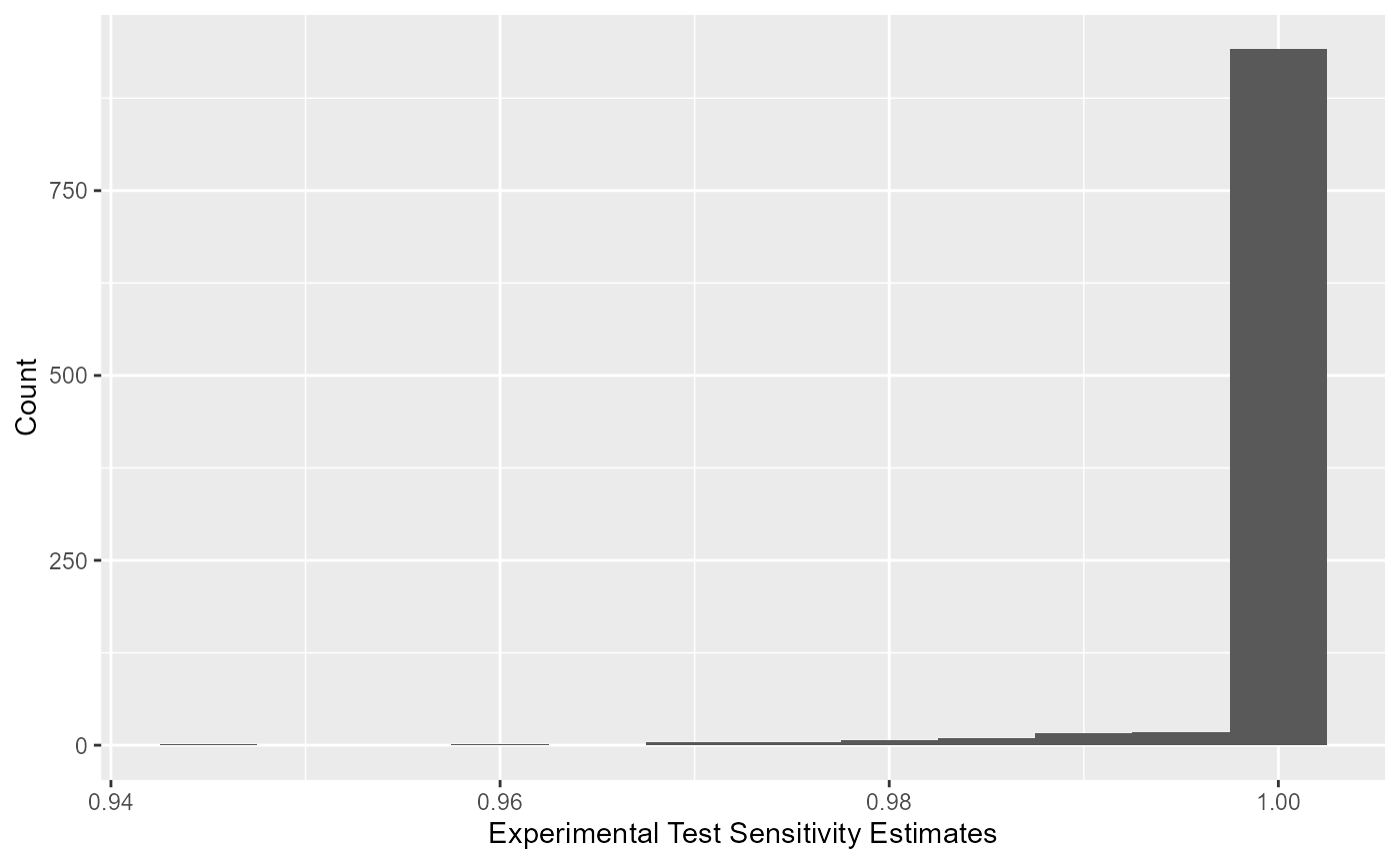
All optimized values for sensitivity of the experimental kit can be viewed using a histogram.

Sn figure

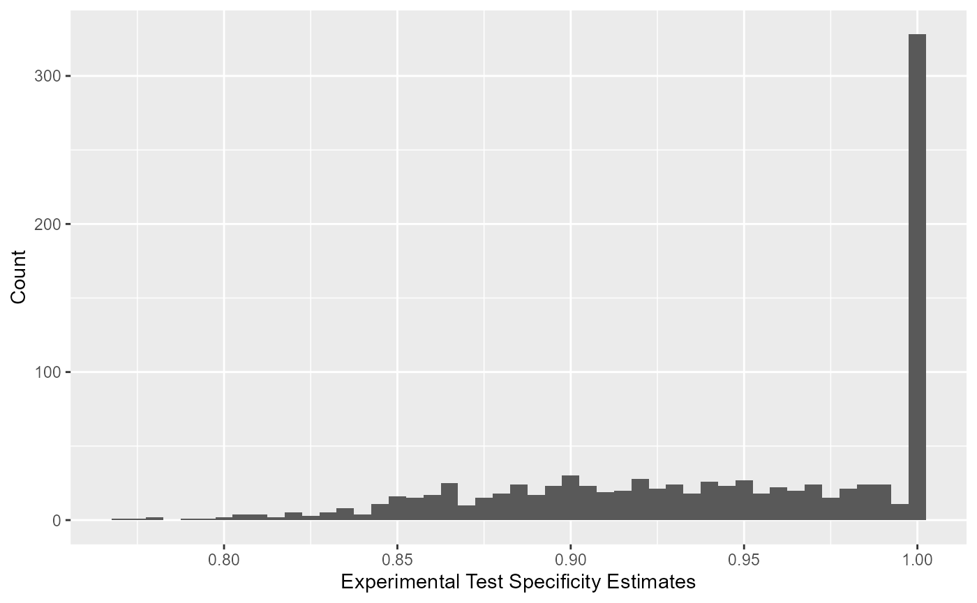
All optimized values for specificity of the experimental kit can be viewed using a histogram.

Sp figure

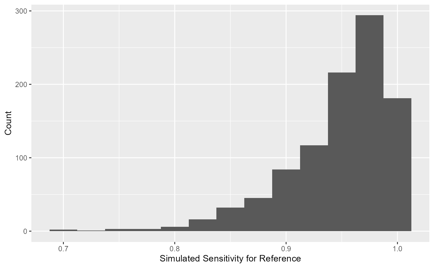
Simulated Values for Reference Test

Similarly, the simulated values of sensitivity for the reference test can be extracted using blood_SnSp$input$Sn.sims. The simulated distribution for the sensitivity of the reference test is displayed as a histogram.

Sn reference

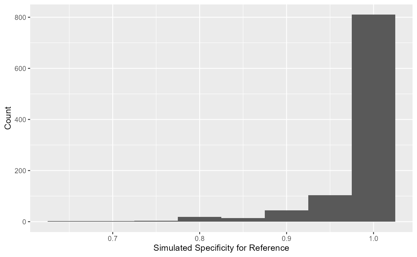
The simulated values of specificity for the reference test can be extracted using blood_SnSp$input$Sp.sims. The simulated distribution for the specificity of the reference is displayed as a histogram.

Sp reference

#Infallible Reference Test

Use the cloppearSnSp function to estimate the sensitivity and specificity of a 2–state experimental test when an infallible reference test has been used to determine the true disease status of each sample. The function has one required input, the data frame of counts (dat).

Estimating Sensitivity

By default the function will estimate sensitivity.

infal_Sn <- cloppearSnSp(dat = infallible)
infal_Sn

## [1] "Sn = P(T+|D+): 0.987013 (95% CI: 0.953876, 0.998423)"

The total number of positive samples tested can be extracted using infal_Sn$data$Total.Positive and the number of positive samples that tested positive by the experimental test can be obtained using infal_Sn$data$Test.Positive. The sensitivity estimate can be obtained by infal_Sn$calcVal$Sn and the lower and upper confidence limits can be obtained using infal_Sn$calcVal$Sn.LL and infal_Sn$calcVal$Sn.UL, respectively.

Estimating Specificity

The function will estimate specificity when est.Sn = FALSE.

infal_Sp <- cloppearSnSp(dat = infallible,
                         est.Sn = FALSE)
infal_Sp

## [1] "Sp = P(T-|D-): 0.970297 (95% CI: 0.915643, 0.993832)"

Similarly, the total number of negative samples tested can be extracted using infal_Sp$data$Total.Negative and the number of negative samples that tested negative by the experimental test can be obtained using infal_Sp$data$Test.Negative. The specificity estimate can be obtained by infal_Sp$calcVal$Sp and the lower and upper confidence limits can be obtained using infal_Sp$calcVal$Sp.LL and infal_Sp$calcVal$Sp.UL, respectively.